
Applies To
Tip: Try using the new XLOOKUP function, an improved version of VLOOKUP that works in any direction and returns exact matches by default, making it easier and more convenient to use than its predecessor.
Use VLOOKUP when you need to find things in a table or a range by row. For example, look up a price of an automotive part by the part number, or find an employee name based on their employee ID.
In its simplest form, the VLOOKUP function says:
=VLOOKUP(What you want to look up, where you want to look for it, the column number in the range containing the value to return, return an Approximate or Exact match – indicated as 1/TRUE, or 0/FALSE).
Paused
Tips:
- The secret to VLOOKUP is to organize your data so that the value you look up (Fruit) is to the left of the return value (Amount) you want to find.
- If you’re a Microsoft Copilot subscriber Copilot can make it even easier to insert and use VLookup or XLookup functions. See Copilot makes lookups in Excel easy.
Technical details
How to get started
There are four pieces of information that you will need in order to build the VLOOKUP syntax:
- The value you want to look up, also called the lookup value.
- The range where the lookup value is located. Remember that the lookup value should always be in the first column in the range for VLOOKUP to work correctly. For example, if your lookup value is in cell C2 then your range should start with C.
- The column number in the range that contains the return value. For example, if you specify B2:D11 as the range, you should count B as the first column, C as the second, and so on.
- Optionally, you can specify TRUE if you want an approximate match or FALSE if you want an exact match of the return value. If you don’t specify anything, the default value will always be TRUE or approximate match.
Now put all of the above together as follows:
=VLOOKUP(lookup value, range containing the lookup value, the column number in the range containing the return value, Approximate match (TRUE) or Exact match (FALSE)).
Examples
Here are a few examples of VLOOKUP:
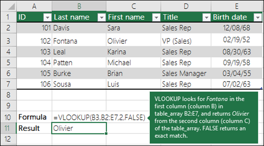
Example 1
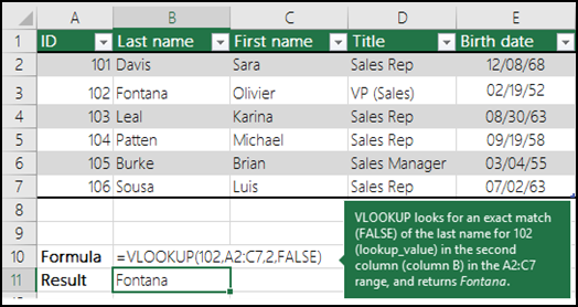
Example 2
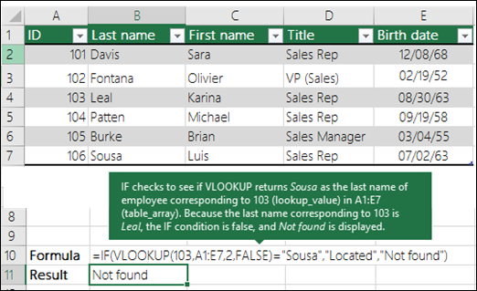
Example 3
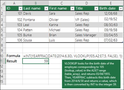
Example 4
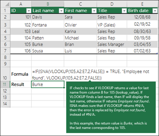
Example 5
Common Problems
Best practices
Need more help?
You can always ask an expert in the Excel Tech Community or get support in Communities.
See Also
Quick Reference Card: VLOOKUP refresher
How to correct a #N/A error in the VLOOKUP function
Look up values with VLOOKUP, INDEX, or MATCH


Need more help?
Want more options?
D